procedural generation techniques - 3d scene that shows examples of procedurally generated content
project timescale: february 2015 - april 2015
Below is the report I wrote on this project.
Introduction
The aim of the project was to make an application that creates and renders a 3D scene with examples of procedural content generation techniques. It also required a post processing effect and an interactive camera that allowed the user to look around the scene.
The created application was made with the Rastertek DirectX 11 framework. It uses various methods to alter a flat plain into interesting terrain. These include; height map generation, faulting, smoothing and cellular automata. With these tools, the terrain can consist of sharp mountains, rolling hills, shallow islands or a combination of the three. The terrain texture changes depending on how steep the terrain is so flat areas look like grass and steep areas look like rock.
Cellular automata was also used to create Conway’s game of life. There is also a dungeon generator that uses binary space partitioning to create rooms and find paths between them. A pixel shader makes use of convolution matrices to create an edge detection post processing effect. The camera included in the Rastertek framework was used for the interactive camera.
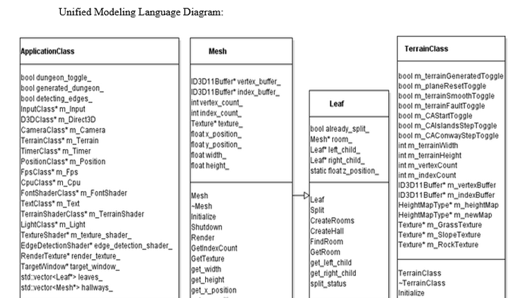
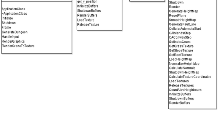
Application Design
The program was planned to be made with the Rastertek framework. The main classes of interest are the application class, terrain class, mesh class and leaf class.
The application class controls the main logic of the program. It handles all the input, renders the objects in the scene and renders the scene to a texture for adding post processing effects. The main object being rendered is the terrain which is rendered with a terrain shader class. The application also generates the dungeons using the leaf class and mesh clash. The leaves and meshes are rendered with a texture shader. The inputs are used to move the camera, manipulate the terrain and generate the dungeons. An edge detection shader class is used to render the scene with an edge detection post processing effect.
The terrain class contains functions that cause the various different changes to the terrain’s geometry. These include smoothing, faulting and cellular automata algorithms. The class also has functions to calculate texture coordinates and normals which are called each time an alteration to the terrain is made. Three different textures are stored in the class which are used by the terrain shader to change the texture at any point on the terrain based on how steep the terrain is at that point.
The mesh class is used to make textured quads of varying dimensions at any position in the scene. These meshes are used to represent the rooms and hallways of the dungeons.
The leaf class inherits from the mesh class. It uses the binary space partitioning method to create dungeons. It has a function that splits itself into 2 smaller leaves as well as functions to create and find rooms for the dungeons and also a function to create halls for the dungeons.
Introduction
The aim of the project was to make an application that creates and renders a 3D scene with examples of procedural content generation techniques. It also required a post processing effect and an interactive camera that allowed the user to look around the scene.
The created application was made with the Rastertek DirectX 11 framework. It uses various methods to alter a flat plain into interesting terrain. These include; height map generation, faulting, smoothing and cellular automata. With these tools, the terrain can consist of sharp mountains, rolling hills, shallow islands or a combination of the three. The terrain texture changes depending on how steep the terrain is so flat areas look like grass and steep areas look like rock.
Cellular automata was also used to create Conway’s game of life. There is also a dungeon generator that uses binary space partitioning to create rooms and find paths between them. A pixel shader makes use of convolution matrices to create an edge detection post processing effect. The camera included in the Rastertek framework was used for the interactive camera.
Application Design
The program was planned to be made with the Rastertek framework. The main classes of interest are the application class, terrain class, mesh class and leaf class.
The application class controls the main logic of the program. It handles all the input, renders the objects in the scene and renders the scene to a texture for adding post processing effects. The main object being rendered is the terrain which is rendered with a terrain shader class. The application also generates the dungeons using the leaf class and mesh clash. The leaves and meshes are rendered with a texture shader. The inputs are used to move the camera, manipulate the terrain and generate the dungeons. An edge detection shader class is used to render the scene with an edge detection post processing effect.
The terrain class contains functions that cause the various different changes to the terrain’s geometry. These include smoothing, faulting and cellular automata algorithms. The class also has functions to calculate texture coordinates and normals which are called each time an alteration to the terrain is made. Three different textures are stored in the class which are used by the terrain shader to change the texture at any point on the terrain based on how steep the terrain is at that point.
The mesh class is used to make textured quads of varying dimensions at any position in the scene. These meshes are used to represent the rooms and hallways of the dungeons.
The leaf class inherits from the mesh class. It uses the binary space partitioning method to create dungeons. It has a function that splits itself into 2 smaller leaves as well as functions to create and find rooms for the dungeons and also a function to create halls for the dungeons.
Techniques Used
To represent a point on the terrain, a struct called HeightMapType was used. This struct contains x, y and z positions, texture coordinates and normals. To represent the whole terrain an array of HeightMapType structs was created.
To generate a random height map, the program would loop through the array and change every y position to be a random value in the range 0-9. This created a very jagged looking terrain.
To reset the terrain, the program would loop through the array and change every y position to 0. This returned the terrain to a flat plain.
For smoothing, the program first got a single point on the terrain. It then got the points immediately above, below, to the left and to the right of this point and calculated the average y position of all five points. This average became the new y position of that point on the terrain. If the point was on the edge of the map, then the program only took the average of four points so it didn’t try to retrieve a point that wasn’t there. Smoothing reduced any sharp edges on the terrain.
Generating fault lines was done by using one of the methods described by Lighthouse 3D (no date). The program would find two random points on the terrain and used them to build a vector. Then it would loop through every point on the terrain, create another vector using this point and the first random point and then calculate the y component of the two vectors’ cross product. If the y component was greater than 0, then a pre-calculated displacement value was added to that point’s y position. If the y component wasn’t greater than 0, then the displacement value was subtracted from the point’s y position. This would make a visible line on the terrain, with the geometry on one side higher than the other. When the fault line generation function was called, it repeated this process for a number of iterations. The number of iterations, as well as constant values for the initial and final displacement, were used to calculate the displacement at each fault. Although these values can be changed for slightly different effects, the application used 1 for the initial displacement, 0.5 for the final displacement and repeated the process for 10 iterations. The displacement for each fault line was calculated by multiplying the difference between the final and initial displacement by the current iteration value over the total number of iterations and adding on the initial displacement. The created effect was that each fault line would be smaller than the last.
A cellular automaton is a simulation where there are a grid of cells that are either alive or dead with a set of rules to govern the state of the cells. The grid is initialised so that a random number of cells are alive or dead. When the simulation is running, it iteratively uses the defined set of rules to change the current state of the cells. The rules are based around taking a cell on the grid and counting the number of neighbouring cells which are alive.
The application used two automatons; one that generates islands and a very famous cellular automaton, called Conway’s game of life, which creates complex patterns. These were implemented using a techniques described by Michael Cook (2013). Each point on the terrain was treated as a cell. The HeightMapType struct also contained a boolean which was used to track if the cells were dead or alive. If a cell was alive, then that point on the terrain was elevated and if a cell was dead, the point was lower. This was done by changing the y position of the point.
For the island generation, the set of rules was as follows:
1. If a cell is alive and has less than 4 alive neighbours, it becomes dead.
2. If a cell is alive and has 4 or more alive neighbours, it stays alive.
3. If a cell is dead and has more than 4 alive neighbours, it becomes alive.
4. If a cell is dead and has 4 or less alive neighbours, it stays dead.
For Conway’s game of life, the set of rules was as follows:
1. If a cell is alive and has less than 2 alive neighbours, it becomes dead.
2. If a cell is alive and has 2 or 3 alive neighbours, it stays alive.
3. If a cell is alive and has more than 3 alive neighbours, it becomes dead.
4. If a cell is dead and has 3 alive neighbours, it becomes alive.
A function was used to initialise the grid by looping through every cell and generating a random number from 0 – 100. If the number was less than 45, the cell’s state was set to alive. Two other functions were used to run the simulation step of each automaton using the different rule sets. During a simulation step, the program looped through every cell on the grid and found out how many of that cells’ neighbours were alive. It then checked the rules to see if that cell should be alive or dead. To avoid messing up the neighbour count for other cells, rather than change the cell’s state whilst it was still looping through the grid, the program stored the new state of the cell in another grid. After the loop finished, the cells of the grid were changed to make them match the state of the cells in the other grid.
After a few simulation steps of the island generating automaton, the terrain had some nice looking shallow islands and would no longer change if further steps were made. Repeatedly stepping through the game of life automaton, caused different patterns to occur on the terrain.
The application generated 2D dungeons using binary space partitioning as described by Timothy Hely (2013). Binary space partitioning (BSP) is a technique used to divide up an area into smaller pieces. This can be used for creating dungeons by placing a room in each of the smaller areas and then connecting them with hallways. BSP is an iterative process and keeps splitting areas (called leaves) in two until every leaf has dimensions between the defined maximum and minimum sizes.
The application class contained a vector which stored instances of the leaf class. A root leaf was created and pushed onto the vector. The program would then start a while loop to split leaves, that ended when every leaf had been reduced to appropriate dimensions. In this loop, another loop was used to go through every leaf currently in the vector and see if it needed to be split. A split would occur if the leaf hadn’t already been split and its width or height was greater than the maximum size. There was also a 75% chance of a split occurring, providing this didn’t result in a leaf smaller than the minimum size, to create more variation in the leaves.
To determine if a leaf should split horizontally or vertically, its width and height were compared. If the width was more than twenty five percent larger than the height, it would split vertically or if the height was more than twenty five percent larger than the width, it would split horizontally. If neither of these conditions were true, it would choose the orientation at random. Next, the program would work out the sizes of the two new leaves. First it would get the biggest size these new leaves could be after splitting by subtracting the minimum size from either the width or height, depending on the orientation of the split. Secondly, it determined the distance from the origin to the split by getting a random number between the minimum leaf size and the calculated biggest size these leaves could be. Then the program would create the two child leaves, making the first one the size of the calculated distance and the second one the distance minus the original leaf’s size. These leaves were then added to the vector.
To create the rooms, the program would start at the root leaf and check if its child leaves existed. It would then check if the children had child leaves and then check their children and repeat this until every leaf had been checked. If a leaf had no children then a room was placed in it. The room’s dimensions were determined by getting a random width and height that were less than the width and height of the room and greater than the defined minimum room size. The room was placed at a random point within the leaf that didn’t cause the room to go out of bounds of the leaf.
When checking for existing children, if a leaf had children then the application would iteratively check the descendants of each child until it found two leaves that each contained a room. It would then create a hallway between the two rooms. To do this, the program got a random position in each room. It then got the dimensions of the halls by finding the difference between the x coordinates and between the y coordinates. If the width or height were equal to 0 then the 2 positions are in line and one mesh was created for the hallway. Otherwise two meshes were created and the hallway would have a turn in it, rather than being straight. In the more common case of two meshes, the hallway could take two possible paths. For example right, then up or up, then right. Which path the hallway should take, was determined randomly. After creating the meshes, they were added to a vector that stored all the hallways.
To render the rooms, the program would loop through the vector of leaves and if a leaf had a room, it would render the room with the texture shader. To render the hallways, the program looped through the vector of hallways and rendered them all, also using the texture shader.
The application worked out how steep the terrain was at any given point, to determine how it should be textured as explained by Rastertek (no date). The terrain class contained three different textures; grass, slope and rock. The desired effect was that where the terrain was flat it would look grassy, where it was completely vertical it would look rocky and where it was at an incline it would be a mixture of the other two. In the terrain’s pixel shader the textures were sampled and the sloping factor was calculated subtracting the y normal from 1.
A texture colour was determined by the value of the sloping factor and the final colour returned by the pixel shader was multiplied by the texture colour before being returned. If the sloping factor was less than 0.2 a linear interpolation was performed between the grass colour and slope colour using a blend amount that was calculated by dividing the sloping factor by 0.2. The result of this was used as the texture colour. If the sloping factor was between 0.2 and 0.7 then the texture colour was calculated by performing a linear interpolation between the slope colour and rock colour using a blend amount calculated by subtracting 0.2 from the sloping factor and multiplying by 2. If the sloping factor was greater than 0.7 then the texture colour would be the rock colour.
For a post processing effect, an edge detection shader was implemented based of a shader written by Luke Lee (2013). Two convolution matrices were created that stored values for the x and y components of the desired effect. The shader would loop through both matrices and multiply the colour by the current matrices’ values. It would add the result to the line colours. After the loops finished, the final colour was calculated by getting the square root of the line colours.
User Guide
When the application is run the scene will initially consist of a flat plane in front of the camera with some basic lighting. The user can navigate the scene by moving the camera. The up arrow key moves the camera forwards, the down arrow key moves it backwards, the left arrow key turns it left, the right arrow key turns it right, the A key moves it upwards, the Z key moves it downwards, the PGUP key turns it upwards and the PGDN key turns it downwards.
Pressing the M key generates a 2D dungeon in front of the plane. It is recommended that this is done before moving because you can only view the dungeons from the front.
A random height map field is generated by pressing the space bar. This makes the plane jagged and uneven. Pressing the F key generates a series of fault lines on the plane. A few presses will give the appearance of hills on the terrain but several presses will make it more mountainous looking. Pressing the S key smoothens the plane so that the terrain has softer edges.
The user can initialise the plane for cellular automata algorithms by pressing the C key. After the C key is pressed, the user can either press the V key repeatedly to gradually generate shallow islands on the plane or they can hold the G key to create Conway’s game of life on the terrain. Conway’s game of life is best seen from a bird’s eye view so it is recommended to move the camera high above the terrain and aim it directly down when using this feature.
The plane can be reset to its initial flat appearance at any time by pressing the I key.
Edge detection can be turned on and off by pressing the E key. It is recommended that this is done after faulting so that there are clear edges to see. Otherwise the user is likely to just see white space.
Critical Analyse
The cellular automaton for island generation used 4 as both its birth limit and its death limit. By making both of these values alterable by the user, a greater range of effects could be done to the terrain. These include making the islands smaller and less frequent of making the terrain appear more cavernous.
When the cellular automaton grid was initialised, there is 45 percent chance of the cells being dead or alive. This works well for island generation but if the states of the cells were completely random then a greater range of possible patterns would have emerged in Conway’s game of life. Having two different initialisation functions would have gotten around this problem.
When Conway’s game of life was running, the frame rate of the program drastically slowed. This was probably due to constantly changing the geometry as it was getting rendered. Also the simulation isn’t very clear to see in the 3D geometry of the terrain. Using a 2D grid would have looked a lot better and most likely run more smoothly.
A problem with the dungeons was that some of the hallways would break when they turned. This only occurred when the path of a hallway went up and left. It is unknown what caused this minor issue.
For the texturing of the terrain, textures created by Rubberduck (2013) were used. These textures didn’t match so as a result the texturing looks a bit off. The techniques used do work though and with matching textures the affect would be a lot better.
References
Lighthouse 3D. [no date]. Terrain Tutorial The Fault Algorithm. [online] Available from: http://www.lighthouse3d.com/opengl/terrain/index.php3?fault [Accessed 23 January 2015]
Rastertek. [no date]. Tutorial 14: Slope Based Texturing. [online] Available from: http://www.rastertek.com/tertut14.html [Accessed 7 April 2015]
Rubberduck. 2013. 50 free textures [digital images] [Viewed 7 April 2015]. Available from: http://opengameart.org/content/50-free-textures
Cook, M. 2013. Generate Random Caves Using Cellular Automata. [online] Available from: http://gamedevelopment.tutsplus.com/tutorials/generate-random-cave-levels-using-cellular-automata--gamedev-9664 [Accessed 19 February 2015]
Hely, T. 2013. How to Use BSP Trees to Generate Game Maps. [online] Available from: http://gamedevelopment.tutsplus.com/tutorials/how-to-use-bsp-trees-to-generate-game-maps--gamedev-12268 [Accessed 4 March 2015]
Lee, L. 2013. HLSL Edge Detection Effect. [online] Available from: http://lukelook.com/?portfolio=hlsl-edge-detection-effect [Accessed 8 April 2015]
